How smart data analysis can help you save on real estate costs | Deephaven

Efficient real estate data analysis is essential for investors, homeowners, and renters to understand the market and find appropriate properties to buy or rent. This article will demonstrate how Deephaven can help you with large amounts of data to make informed decisions. Deephaven simplifies gathering and analyzing static and real-time data, so users can perform their own research easily and flexibly.

As an example, we will use the Nasdaq Data Link API to get the Zillow data feed that contains real estate indicators, such as market indices, rental, sales, and inventories for thousands of areas across the US. When analyzing the housing market, one of the most popular metrics one should consider is the price-to-rent ratio. Homeowners and renters use it to decide whether to buy or rent. Real estate investors use this ratio to analyze investment opportunities and find the most cost-effective properties.

In this blog, we will look at the Boston area and demonstrate how to uncover insights about rental and sales values from the comfort of your home in a matter of minutes.

To calculate the price-to-rent ratio using Deephaven tables, you just need to follow a few steps:

1. Import a few libraries:

os.system("pip install nasdaq-data-link")

import numpy as np
import pandas as pd
import nasdaqdatalink
from deephaven import SortDirection
from deephaven import pandas as dhpd
from deephaven.plot.figure import Figure

2. Create a free account on Nasdaq Data Link and save your API key to a variable:

nasdaqdatalink.ApiConfig.api_key = '<INSERT YOUR KEY HERE>'

3. Get the list of regions from the ZILLOW/REGIONS table:

df_regions = nasdaqdatalink.get_table("ZILLOW/REGIONS", paginate=True)


df_regions = df_regions[df_regions["region_type"] == "zip"]


regions = dhpd.to_table(df_regions)
regions = regions.update(["region_type = (String)region_type", "region = (String)region", "region_id = (String)region_id"])

4. The region column has multiple location elements separated by a semicolon. Let’s split this column up:

units = ["zip", "state", "metro", "county", "city"]
df_regions[units] = df_regions["region"].str.split('; ', expand=True)
for unit in units:
    values = list(df_regions[unit])
    regions = regions.update([unit + "= (String)values[i]"])

5. In this example, we only want to analyze the Boston-Cambridge-Newton area, so we need to limit the list to those region ids:

regions = regions.where(filters=["metro = `Boston-Cambridge-Newton`"])


distinct_region_ids = regions.select_distinct(formulas=["region_id"])
list_of_regions = dhpd.to_pandas(distinct_region_ids)['region_id'].tolist()

6. Now we can get the median home price and median rent from the Nasdaq Data Link API:

df_region_price = nasdaqdatalink.get_table("ZILLOW/DATA", paginate=True, indicator_id='ZALL', region_id=list_of_regions)


region_price = dhpd.to_table(df_region_price)
region_price = region_price.update(["indicator_id = (String)indicator_id", "region_id = (String)region_id", "median_price = (double)value", "date = (DateTime)date"])


df_region_rent = nasdaqdatalink.get_table("ZILLOW/DATA", paginate=True, indicator_id='RSSA', region_id=list_of_regions)

region_rent = dhpd.to_table(df_region_rent)
region_rent = region_rent.update(["indicator_id = (String)indicator_id", "region_id = (String)region_id", "median_rent = (double)value", "date = (DateTime)date"])

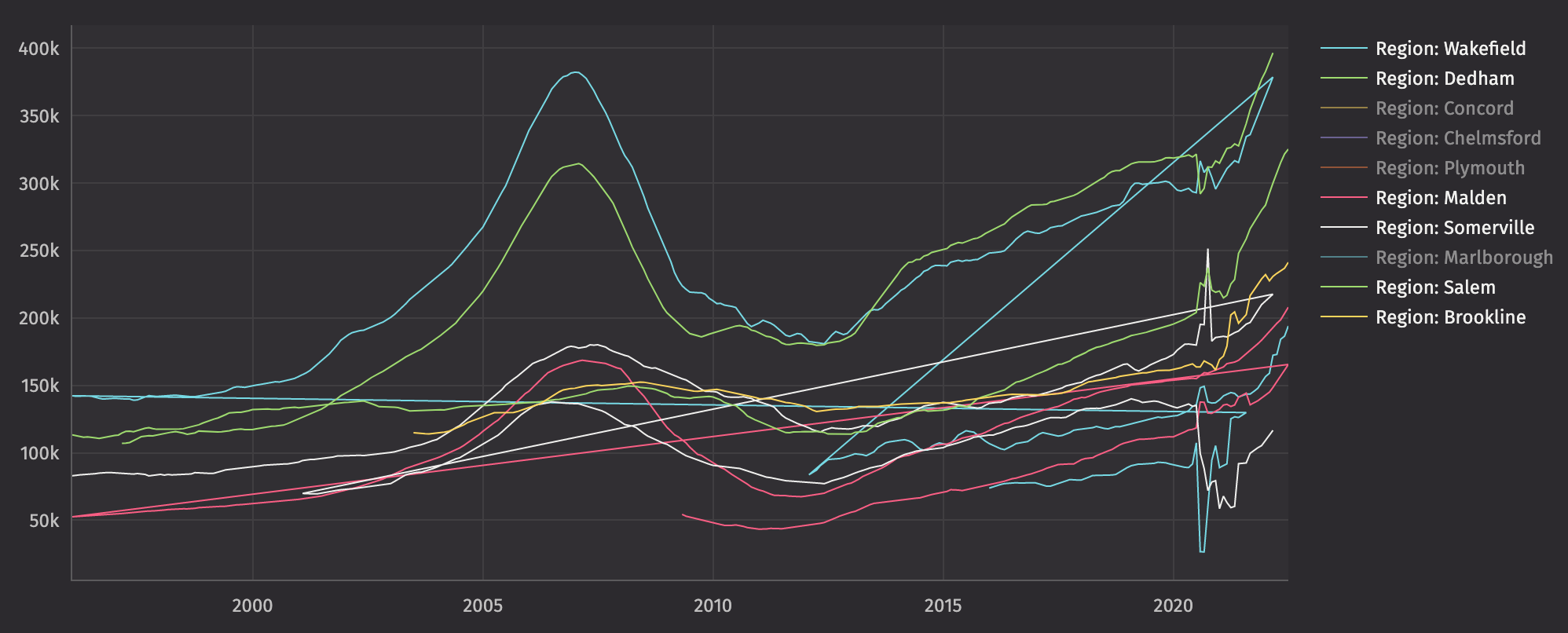
7. It will be interesting to look into the historical trend of home prices between 2000 and 2020 and compare a few regions over this period of time, and we can easily do this by creating an XY plot with multiple series:

figure = Figure()
table = region_price.join(table=regions, on=["region_id"], joins=["city"])
trend_chart = figure.plot_xy(series_name="Region", t=table, x="date", y="median_price", by=["city"]).show()

8. Merge all the tables:

indicators = region_price.join(table=region_rent, on=["region_id"], joins=["median_rent"])


table = indicators.join(table=regions, on=["region_id"], joins=["zip", "state", "county", "city", "metro"])

9. Calculate PRR:

table = table.update(formulas=["PRR = median_price / (median_rent * 12)"])

If the price-to-rent ratio is 15 or less, buying is better than renting. Our area’s ratio is even greater than 60, so renting makes more financial sense!

10. Aggregate data by city and build a column chart to visualize the results in descending order:

table_by_city = table.select(formulas=["city", "PRR"]).avg_by(by=["city"])
table_by_city = table_by_city.sort(order_by=["PRR"], order=[SortDirection.DESCENDING])
figure = Figure()
new_f = figure.plot_cat(series_name="city", t=table_by_city, category="city", y="PRR")
plot1 = new_f.show()

The Zillow real estate data feed we used is updated every week, but you might want to get the latest information about the real estate market to examine the current trends. To receive the most accurate and updated information, you can use multiple real-time MLS listings, which provide a feed of information about homes long before websites like Zillow or Realtor.com. Deephaven tables operate the same way regardless of whether the data is batch or streaming. The methods we use to calculate the price-rent ratio remain the same!

Our example provided a basic starter, but you can use it to make your own analysis. If you have similar use cases or want to share your ideas, we’d love to hear about them! Reach out to us on Slack.