Large Language Models and Nearest Neighbors

Instead of jumping on the latest trend of the week, I wanted to dive into a recent, fascinating application of nearest-neighbor methods in the context of large language models (LLMs) that made big waves in July.

You may know that I like simple yet elegant and baselines, but I also found this method quite refreshing given that most of the current research is about scaling already massive LLMs. While they may not scale to all kinds of problems where LLMs currently excel, seemingly simple methods such as nearest neighbor algorithms have a certain beauty to them. It also shows that there are still many opportunities to innovate and make significant contributions based on foundational or “classic” techniques.

Nearest neighbor methods are one of the fundamental methods in data mining, pattern recognition, and machine learning. They are used in classification and regression tasks, as well as in recommendation systems, anomaly detection, and other applications.

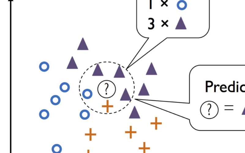
The most basic form of a nearest neighbor method is the k-nearest neighbors (kNN) algorithm. When classifying a new point, the kNN algorithm looks at the k points in the training data nearest to the new point — k is a hyperparameter chosen by the user. The new point is then classified based on a majority vote of these neighbors. If the majority of these neighbors belong to a specific class, then the new point is assigned to that class, as illustrated ion the figure below.

Notably, no training is involved since for each new data point to classify, we just need to identify the k-nearest neighbors in the training set. (The downside is that each prediction requires iterating over the training set, which is expensive for larger training sets.)

This is essentially all you need to know about kNN to understand the paper below. However, if you are interested in further details, I included information and further resources, including methods for improving efficiency, at the bottom of this article.

I talked a bit about the “Low-Resource” Text Classification: A Parameter-Free Classification Method with Compressors paper on my social channels when it made big waves at ACL 2023 a few weeks ago — I was attending the SciPy 2023 conference during this time, and it was also the topic at several dinner conversations there as well.

However, I didn’t include it in the previous AI Research Highlights In 3 Sentences Or Less issue since it was technically based on the Less is More: Parameter-Free Text Classification with Gzip paper posted on arXiv in December 2022, which may have been part of a previous conference submission.

Anyways, let’s dive in and see what this “Low-Resource” Text Classification: A Parameter-Free Classification Method with Compressors paper is all about.

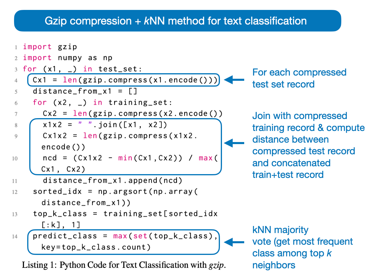
In short, the “Low-Resource” Text Classification paper aims to classify texts using gzip (the compression format and tool) and kNN. The method is summarized via the following Python code in the annotated figure below.

Here, ncd stands for Normalized Compression Distance, a similarity measure between two strings based on the length of their compressed forms. It is calculated by compressing the individual strings and their concatenation, comparing compression lengths to produce a score ranging from 0 (identical strings) to 1 (no similarity). (A step-by-step explanation will follow in the next section.)

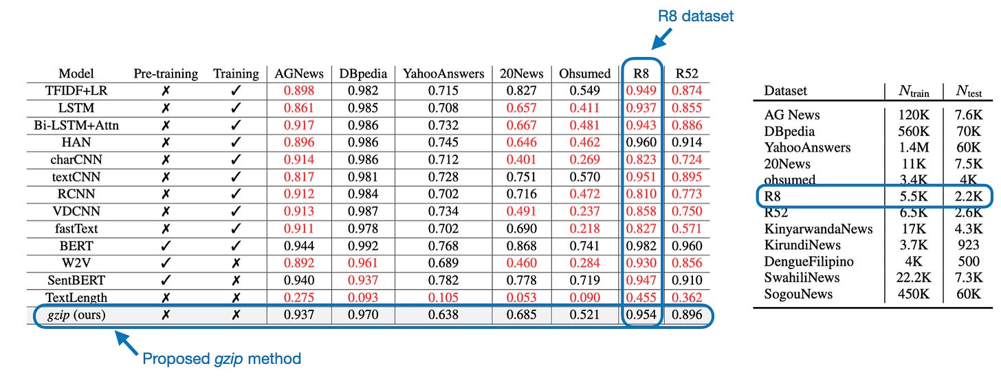
Surprisingly, this method is very competitive, and the classification performance is almost as good as BERT (an encoder-style LLM; discussed in Understanding Encoder And Decoder LLMs) on several datasets, as shown in the table below.

Regarding out-of-distribution (OOD) classification and few-shot settings, the proposed gzip method outperforms BERT and all other methods, as shown below. (OOD here means that the BERT finetuning and classification are done on datasets in languages not seen by BERT during pretraining.)

Note that these numbers are slightly inflated due to a coding bug, but we will get to this later. First, let’s go over how this method fundamentally works.

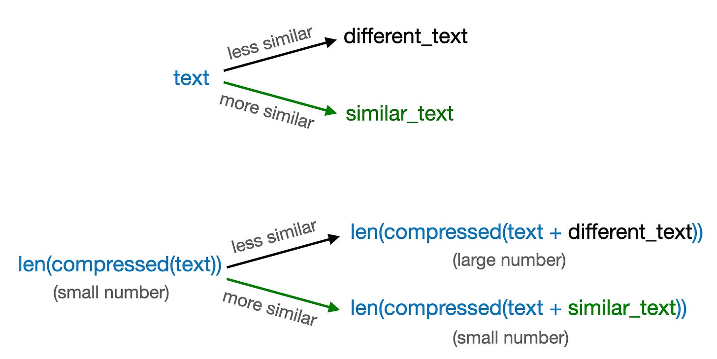
On a high level, the proposed gzip method leverages the fact that compression algorithms remove redundant information.

For instance, when compressed, text 1 is close to the size of two concatenated texts, text 1 and text 2, if these texts are similar. Or, consider this more extreme case: the compressed size of a text concatenated with itself is similar to the size of the original compressed text (plus a small constant value for the back reference).

Sounds complicated? Let’s walk through it step by step using actual Python code. Suppose we have the following two texts:

txt_1 = "hello world"

txt_2 = "some text some text some text"

Let’s compress it using gzip and return the lengths of the compressed strings:

>>> import gzip
>>> len(gzip.compress(txt_1.encode()))
31
>>> len(gzip.compress(txt_2.encode()))
33

We can see that the second compressed text has approximately the same size as the first compressed text, even though the second compressed text is significantly longer. Here, the compression algorithm may take advantage of the fact that some of the text in txt_2 is repeated.

Let’s now concatenate text 1 and text 2 and see what happens when the concatenated text is compressed:

>>> len(gzip.compress(" ".join([txt_1, txt_2]).encode()))
43

We can see that the concatenated text is now noticeably longer than any of the two individual texts, which is expected since the two texts are quite different.

In contrast, if we concatenate each text with itself, the compressed version is almost identical in length to the non-concatenated compressed text:

>>> len(gzip.compress(" ".join([txt_1, txt_1]).encode()))
34

>>> len(gzip.compress(" ".join([txt_2, txt_2]).encode()))
33

Note that concatenating a text with itself is an extreme case. The general idea is that the length of a compressed text is more similar to a text concatenated to a similar text versus a different text when compressed, as summarized in the figure below.

The authors shared a GitHub repository implementing the experiments from the paper. However, in this section, we will reimplement the method based on how it was described in the paper and apply it to sentiment classification in the IMDB Movie Review dataset, which was not part of the original study.

Code Repository

I made all the code for these experiments below available at https://github.com/rasbt/nn_plus_gzip.

The IMDB movie review dataset, in the way I partitioned it below, consists of 35,000 training examples, and 10,000 examples for testing:

import pandas as pd

from local_dataset_utilities import download_dataset, load_dataset_into_to_dataframe, partition_dataset

df_train = pd.read_csv("train.csv")
df_val = pd.read_csv("val.csv")
df_test = pd.read_csv("test.csv")

(The local_datasets_utilities can be found here.)

The baseline accuracy (always predicting the majority class) for the binary classification task (predicting whether a movie review is positive or negative) is 50.06% since the dataset is balanced:

>>> bcnt = np.bincount(df_test["label"].values)
>>> print(bcnt)
array([5006, 4994])

>>> print("Baseline accuracy:", np.max(bcnt)/ bcnt.sum())
Baseline accuracy: 0.5006

Now, based on the Python code from the paper shown again below,

we can implement the gzip method as follows:

import gzip
import numpy as np
from tqdm import tqdm

k = 2
predicted_classes = []

for row_test in tqdm(df_test.iterrows(), total=df_test.shape[0]):
    test_text = row_test[1]["text"]
    test_label = row_test[1]["label"]
    c_test_text = len(gzip.compress(test_text.encode()))
    distance_from_test_instance = []
    
    for row_train in df_train.iterrows():
        train_text = row_train[1]["text"]
        train_label = row_train[1]["label"]
        c_train_text = len(gzip.compress(train_text.encode()))
        
        train_plus_test = " ".join([test_text, train_text])
        c_train_plus_test = len(gzip.compress(train_plus_test.encode()))
        
        ncd = ( (c_train_plus_test - min(c_train_text, c_test_text))
                / max(c_test_text, c_train_text) )
        distance_from_test_instance.append(ncd)
        
    sorted_idx = np.argsort(np.array(distance_from_test_instance))
    
    top_k_class = list(df_train.iloc[sorted_idx[:k]]["label"].values)
    predicted_class = max(set(top_k_class), key=top_k_class.count)
    predicted_classes.append(predicted_class)

print("Accuracy:", np.mean(np.array(predicted_classes) == df_test["label"].values))

This code runs for about a day and reaches and accuracy of 70.05% (1_1_nn_plus_gzip_original.ipynb). Note that we set k=2 and did not preprocess the data, which are both settings the authors used in the original paper for all experiments as well.

In practice, there’s a slight problem when using k=2, for instance, how do we break ties if the labels of the two nearest neighbors are [0, 1] or [1, 0]?

Using the code provided in the paper, the method always selects the lowest class label index in case of a tie. Or in other words, the method is biased toward the class label 0:

>>> top_k_class = [0, 1]
>>> max(set(top_k_class), key=top_k_class.count))
0
​
>>> top_k_class = [1, 0]
>>> max(set(top_k_class), key=top_k_class.count)
0
​
>>> top_k_class = [1, 0, 2]
>>> max(set(top_k_class), key=top_k_class.count)
0

A better way to break ties is always to select the closer neighbor. We can achieve this using a Counter object, as shown below. Here, assume the labels are sorted in ascending order based on the nearest-neighbor distances toward the data point we want to classify.

>>> from collections import Counter
>>> top_k_class = [0, 1]
>>> Counter(top_k_class).most_common()[0][0]
0
​
>>> top_k_class = [1, 0]
>>> Counter(top_k_class).most_common()[0][0]
1
​
>>> top_k_class = [1, 2, 0]
>>> Counter(top_k_class).most_common()[0][0]
1

Using this improved tie-breaking method, we can now update the code as follows:

from tqdm import tqdm
from collections import Counter
​
k = 2
​
predicted_classes = []
​
for row_test in tqdm(df_test.iterrows(), total=df_test.shape[0]):
   test_text = row_test[1]["text"]
   test_label = row_test[1]["label"]
   c_test_text = len(gzip.compress(test_text.encode()))
   distance_from_test_instance = []
   
   for row_train in df_train.iterrows():
       train_text = row_train[1]["text"]
       train_label = row_train[1]["label"]
       c_train_text = len(gzip.compress(train_text.encode()))
       
       train_plus_test = " ".join([test_text, train_text])
       c_train_plus_test = len(gzip.compress(train_plus_test.encode()))
       
       ncd = ( (c_train_plus_test - min(c_train_text, c_test_text))
               / max(c_test_text, c_train_text) )
       distance_from_test_instance.append(ncd)
       
   sorted_idx = np.argsort(np.array(distance_from_test_instance))
   top_k_class = np.array(df_train["label"])[sorted_idx[:k]]
   predicted_class = Counter(top_k_class).most_common()[0][0]
   
   predicted_classes.append(predicted_class)
       
print("Accuracy:", np.mean(np.array(predicted_classes) == df_test["label"].values))

This improves the accuracy from 70.05% (1_1_nn_plus_gzip_original.ipynb) to 71.91% (1_2_nn_plus_gzip_fix-tie-breaking.ipynb).

Note: I also added a more efficient implementation (1_2_caching-multiprocessing.py) caching the compressed training instances and parallelizing the search across different GPU cores. On a MacBook Air, this reduces the runtime from 12h to 2h on the IMDb Movie review dataset.

I chose the IMDB Movie Review dataset for my experiments because I am relatively familiar with it based on other projects I worked on in the past. For example, here are some numbers from my Machine Learning with PyTorch and Scikit-Learn book:

Using the code implementation from my Deep Learning Fundamentals Course, someone even achieved

Another interesting baseline would be to select similar word-count vectors from a bag-of-words model using kNN. (I covered it in my course here if you want to learn about bag-of-words.) The rationale is that two similar texts should have similar count vectors. So, instead of comparing the length of a compressed text to the length of a compressed concatenation of two texts, we could use word count vectors.

If we have a word count vector of text 1 and a count vector of text 2, with similar texts, the two added count vectors should be similar. For example, suppose we have the following count vectors of two identical texts:

text_1 = [0, 3, 1]
text_2 = [0, 3, 1]

Then, the added count vectors are [0, 3, 1] + [0, 3, 1] = [0, 6, 2] = 2 * [0, 3, 1]. So, if we normalize the count vectors before and after adding the counts should be exactly the same:

import numpy as np
​
>>> text_1 = np.array([0., 3., 1.]) 
>>> text_2 = np.array([0., 3., 1.])
​
>>> text_1 /= np.sum(text_1)
>>> print(text_1)
[0.   0.75 0.25]
​
>>> text_2 /= np.sum(text_2)
>>> print(text_2)
[0.   0.75 0.25]
​
>>> added = text_1 + text_2
>>> print(added / np.sum(added))
[0.   0.75 0.25]

Then, we could compute the distance between two vectors using a Euclidean distance metric:

>>> dist = np.sqrt(np.sum((test_vec - added)**2))

However, instead of doing that, we could also just directly compute the cosine similarity between two vectors, which is essentially the same thing:

>>> from numpy.linalg import norm
>>> cosine = 1 - (np.dot(test_vec, train_vec)
...     /(norm(test_vec)*norm(train_vec)))

(Note that the 1- is required to convert the cosine similarity into a cosine distance.)

The complete code then becomes the following:

from collections import Counter
from tqdm import tqdm
from numpy.linalg import norm
​
​
k = 2
​
predicted_classes = []
​
for i in tqdm(range(df_test.shape[0]), total=df_test.shape[0]):
​
   test_vec = X_test[i].toarray().reshape(-1)
   test_label = df_test.iloc[i]["label"]
   distance_from_test_instance = []
   
   for j in range(df_train.shape[0]):
       train_vec = X_train[j].toarray().reshape(-1)
       train_label = df_train.iloc[j]["label"]
       
       cosine = 1 - np.dot(test_vec, train_vec)/(norm(test_vec)*norm(train_vec))
       distance_from_test_instance.append(cosine)
       
   sorted_idx = np.argsort(np.array(distance_from_test_instance))
   top_k_class = np.array(df_train["label"])[sorted_idx[:k]]
   predicted_class = Counter(top_k_class).most_common()[0][0]
   
   predicted_classes.append(predicted_class)
       
print("Accuracy:", np.mean(np.array(predicted_classes) == df_test["label"].values))

The resulting accuracy is 68.01% (4_r8-dataset.ipynb) which is not as good as the gzip method but close (within 4%)!

Above, we evaluated the gzip method on the IMDB movie review dataset, which was not part of the original paper. So, to see how my reimplementation with the improved tie-breaking strategy fares compared to one of the datasets used in the paper, let’s look at the R8 dataset (I chose this because it’s relatively small and only takes a few minutes to run).

Using the lowest-index tie breaking strategy described in one of the figures in the paper, the accuracy is 88.90% (4_r8-dataset.ipynb), which is lower than reported in the original paper. (Please see the following section for a potential explanation.) In comparison, the performance with the improved tie-breaking strategy I described earlier results in 91.27% — still lower than the one reported in the paper. The next session offers an explanation for this discrepancy.

As Ken Schutte discussed on his website, using k=2 is a bit of an odd choice in the context of resolving ties like [0, 1] or [1, 0]. There are several ways to resolve ties, including

1. always using the lower class index (like it is done in scikit-learn and in the Python code shown in a figure in the original paper);

2. choosing the closer one of the two neighbors (my preferred choice, which I implemented in the Fixing the Tie-Breaking section above);

3. determining the winning label randomly.

As Ken Schutte discussed, the paper’s GitHub repository uses a fourth strategy, which may be related to a coding bug. For instance, it resolves ties by always choosing the correct test label:

# here, sorted_pred_lab[][] has the 
# labels and counts corresponding
# to the top-k samples,
# [[label,count],[label,count],...]
# grouped-by label and sorted by count.
​
most_label = sorted_pred_lab[0][0]
most_count = sorted_pred_lab[0][1]
​
if_right = 0
for pair in sorted_pred_lab:
   # we loop until we drop below 'most_count', ie
   # this for-loop iterates over those classes
   # tied for highest count
   if pair[1] < most_count:
       break
​
   # this says if ANY of those
   # in the tied-set are equal to
   # the test label,
   # it is marked correct (if_right=1)
   if pair[0] == label[i]:
       if_right = 1
       most_label = pair[0]
​
# accumulate results:        
pred.append(most_label)
correct.append(if_right)

According the the analysis by Ken Schutte, after fixing the tie-breaking, “the gzip method went from best-perfoming to worst-performing.”

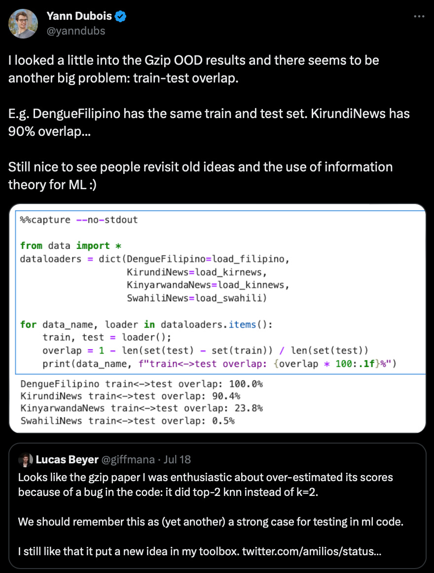
In addition, there also seems to be a dataset overlap, as Yann Dubois shared here:

However, as far as I understand, this overlap more or less affects all methods evaluated in this paper. If you are interested in additional details on the training/test overlap issue, I recommend Ken Schutte’s follow-up post here.

The gzip method proposed in the “Low-Resource” Text Classification: A Parameter-Free Classification Method with Compressors paper is a very elegant, intriguing research contribution. I thoroughly enjoyed exploring it.

Unfortunately, the actual predictive performance of the method may be worse than reported, but it’s an interesting approach nonetheless.

Should we use it in practice? On the one hand, this method has a lot going for it since it’s a simple baseline and doesn’t require GPUs, which is a big plus, given the current GPU shortage. On the other hand, the results are, of course, not as good as advertised, and kNN also doesn’t necessarily scale well to larger datasets — for reference, my naive implementation on IMDb took one day to complete, running on a single CPU.

The positive takeaway here is that we have a new, simple baseline method. And the associated paper highlights why sharing source code and community discussion are so important in disseminating the work (as opposed to just classic peer review).

Below are a few other articles on this topic that I enjoyed reading:

Nearest neighbor algorithms are among the “simplest” supervised machine learning algorithms and have been well-studied in pattern recognition over the last century. While nearest-neighbor algorithms are not as popular as they once were, they are still widely used in practice. I highly recommend that you consider the k-Nearest Neighbor algorithm in classification projects as a predictive performance benchmark, especially when developing more sophisticated models.

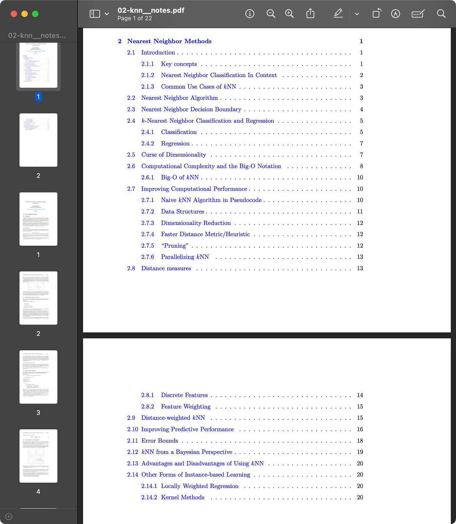
Suppose you want to learn more about nearest-neighbor methods, including k-nearest neighbors. In that case, I have a 20-page lecture note document I’ve written for a machine learning class I taught a few years ago.

But even if you are already familiar with the basics, you might like Section 2.7 on Improving Computational Performance, which includes subsections that could come in handy in practical machine learning and machine learning interviews:

• Using a Priority Queue

• Data Structures: Bucketing, KD-Tree, Ball-Tree

• Dimensionality Reduction

• Faster Distance Metrics & Heuristics

• Pruning

• and Parallelizing kNN

You can find the lecture notes here at https://sebastianraschka.com/pdf/lecture-notes/stat451fs20/02-knn__notes.pdf.

This magazine is personal passion project that does not offer direct compensation. However, for those who wish to support me, please consider purchasing a copy of one of my books. If you find them insightful and beneficial, please feel free to recommend them to your friends and colleagues.

Your support means a great deal! Thank you!