Hedging systematic risk with the Deephaven-IB plugin | Deephaven

Deephaven’s recent release of our Interactive Brokers plugin
brings the power of our professional-grade real-time data engine to all Interactive Brokers users. Today, we’ll
demonstrate how to evaluate beta exposure in Deephaven, using real-time market data from Interactive Brokers.

Beta exposure is an important metric for evaluating systematic risk.
As we’ll see, Deephaven makes it easy to combine live data, historical data, and custom analysis in Python to generate
actionable insights about a trading portfolio. Once we pull it all together, we can keep an eye on everything as it
updates in the Deephaven UI.

Let’s fire up Deephaven with the Interactive Brokers plugin
and get started.

Once Deephaven is running, we can head to http://localhost:10000 and start writing code.
First, we’ll open an API client connection:

API_PORT = 7497

import deephaven_ib as dhib
client = dhib.IbSessionTws(host="host.docker.internal", port=API_PORT, read_only=True)
client.connect()

if client.is_connected():
    print('Client connected!')
else:
    raise RuntimeError("Client not connected!")

Once we’re connected, we can find our example portfolio’s current positions in the accounts_position table:

pos = client.tables['accounts_positions'].last_by(['ContractId'])

From the table of positions, we can extract the current positions’ ticker symbols and submit historical data requests for each
of these symbols.

import numpy as np
from deephaven.pandas import to_pandas


pos_syms = pos.select_distinct(['Symbol'])
mkt_data_syms_set = set(to_pandas(pos_syms)['Symbol'].values)
print('Found ' + str(len(mkt_data_syms_set)) + ' position symbols: ' + str(mkt_data_syms_set))

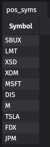
Now we’re ready to request the historical data we need. For this example, we’ll request 253 days of historical
close prices for each of the stocks — enough to calculate a year of returns. In order to calculate betas relative to
the S&P 500, we’ll also retrieve prices for SPY, which is an ETF
that tracks the S&P 500.

mkt_data_syms_set.add('SPY')

from ibapi.contract import Contract
c = Contract()
c.secType = 'STK'
c.exchange = 'SMART'
c.currency = 'USD'

c.symbol = None
for sym in mkt_data_syms_set:
    print('Requesting data for symbol=" + str(sym))
    c.symbol = sym

    rc = client.get_registered_contract(c)
    client.request_bars_historical(
        rc,
        duration=dhib.Duration.days(253),
        bar_size=dhib.BarSize.DAY_1,
        bar_type=dhib.BarDataType.ADJUSTED_LAST,
    )


hist_data_bars = client.tables["bars_historical']

From the historical prices, we can calculate the daily returns:

hist_data_with_return = hist_data_bars.update_view(formulas=[
    'SameTickerAsPrevRow = Symbol=Symbol_[i-1]',
    'Last   = !SameTickerAsPrevRow ? null : Close_[i-1]',
    'Chg    = Close - Last',
    'Return = Chg/Last',
])


spy = hist_data_with_return.where("Symbol=`SPY`")
hist_data_with_spy = hist_data_with_return.natural_join(spy, ['Timestamp'], ['SPY_Return=Return'])

With the data set prepared, we are ready to calculate the betas. To do this, we’ll simply
install SciKit-learn
and run a linear regression. We can use a DynamicTableWriter
to store the results back in a Deephaven table, which lets us easily integrate them with other data sets.

print("Installing sklearn...")
import os
os.system("pip install sklearn")
from sklearn.linear_model import LinearRegression


import deephaven.dtypes as dht
from deephaven import DynamicTableWriter
from deephaven.table import Table

table_writer = DynamicTableWriter(
    {"Symbol": dht.string,
     "Beta": dht.double,
     "Intercept": dht.double,
     "R2": dht.double
     }
)
regression_results = table_writer.table


data_partitioned = hist_data_with_spy.partition_by(['Symbol'])

print('Calculating betas...')
for symbol in mkt_data_syms_set:
    print('Calculating beta for ' + symbol + '...')
    returns_for_betas = data_partitioned.get_constituent(symbol) 
        .where(['!isNull(Return)', '!isNull(SPY_Return)'])

    returns_for_betas_df = to_pandas(returns_for_betas)

    reg = LinearRegression()
    X = returns_for_betas_df['SPY_Return'].values.reshape(-1, 1)
    Y = returns_for_betas_df['Return']
    reg.fit(X, Y)
    r2 = reg.score(X, Y).real

    print(symbol + ' coef: ' + str(reg.coef_) +
          '; intercept: ' + str(reg.intercept_) +
          '; R2: ', str(r2))

    
    table_writer.write_row(
        symbol,
        reg.coef_[0],
        reg.intercept_,
        r2
    )
print('Finished calculating betas!')

Beta calculation complete! We can see the regression coefficient, intercept, and R² for each symbol in the regression_results table:

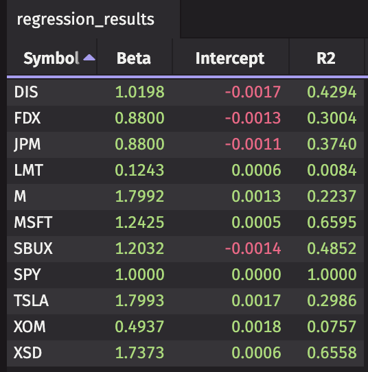
Now it’s time to calculate our portfolio’s beta exposure to SPY. We can use therequest_market_data method to pull the
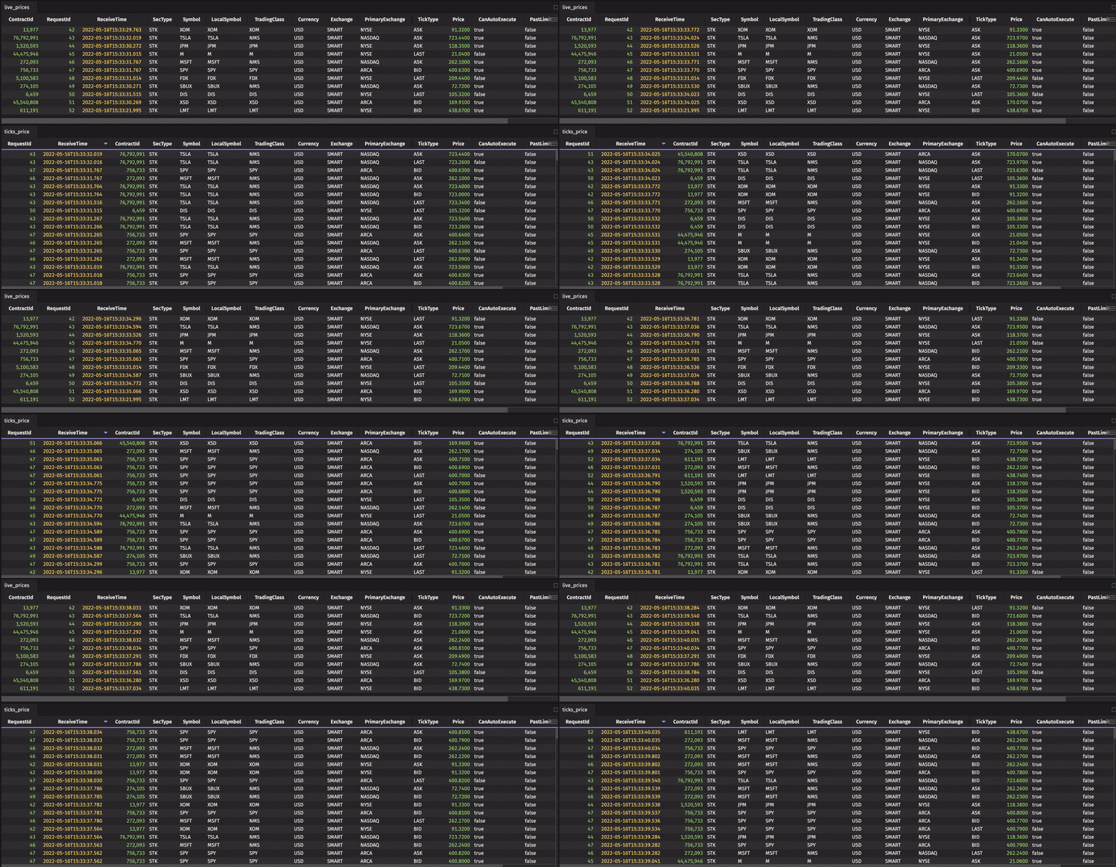
prices for each symbol from Interactive Brokers, which will appear in the ticks_price table from the IB client.
Setting snapshot=False ensures that we are subscribed to real-time data, rather than requesting a one-time snapshot.

After submitting the requests, the prices will continue to update — the ticks_price table will show every tick the
client has received from Interactive Brokers, and the live_prices table will show the latest price for each symbol.

ticks_price = client.tables['ticks_price']
live_prices = ticks_price.last_by(['ContractId'])

for sym in mkt_data_syms_set:
    print('Requesting data for symbol=" + str(sym))
    c.symbol = sym
    rc = client.get_registered_contract(c)
    client.request_market_data(
        rc,
        snapshot=False
    )

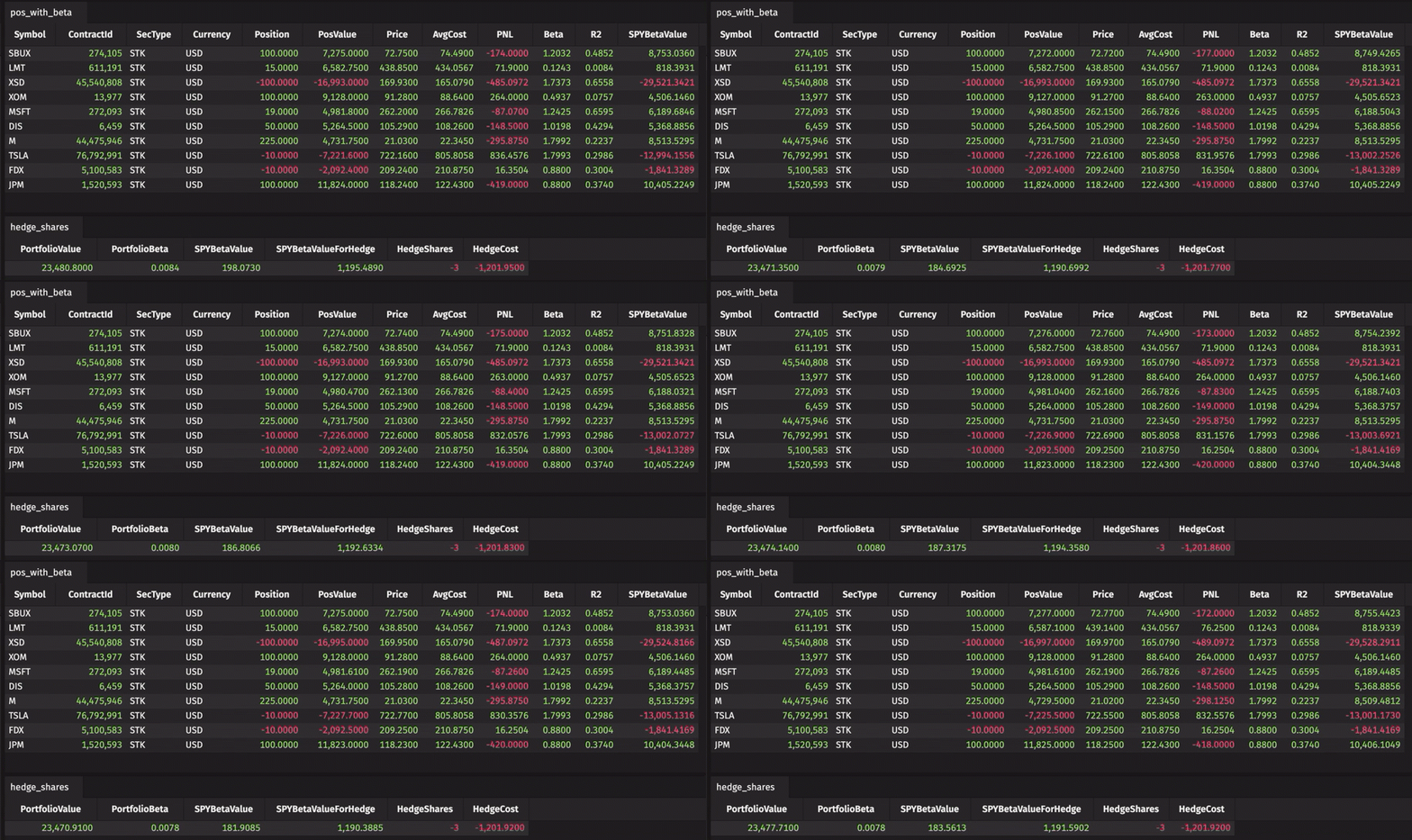
Our three tables of data — betas from historical data, live positions, and live stock prices — are present and populated,
so it”s time to join them together with natural_join.
Since pos table has more columns than we need to see right now, we can also use view to pare down the column set, in addition to calculating three new columns:

1. PosValue — The value of the position in the local currency.
2. PNL — Profit and loss, calculated as the difference between the current PosValue and the total cost of the position.
3. SPYBetaValue — The value of the exposure to SPY, as implied by the modeled beta.

pos_with_beta = pos.natural_join(live_prices, ['ContractId'], ['Price']) 
    .natural_join(regression_results, ['Symbol'], ['Beta', 'R2']) 
    .view([
        'Symbol',
        'ContractId',
        'SecType',
        'Currency',
        'Position',
        'PosValue = Position * Price',
        'Price',
        'AvgCost',
        'PNL = PosValue - AvgCost * Position',
        'Beta',
        'R2',
        'SPYBetaValue = Beta * PosValue',
    ])

Finally, we can calculate the overall beta of the portfolio and evaluate how to hedge it. To do this, we’ll sum up the
position value, dollar-weighted beta, and SPY beta value across the portfolio. For hedging purposes, we’ll exclude
symbols whose beta calculation had a low R², since SPY may not be an effective hedge for these positions.

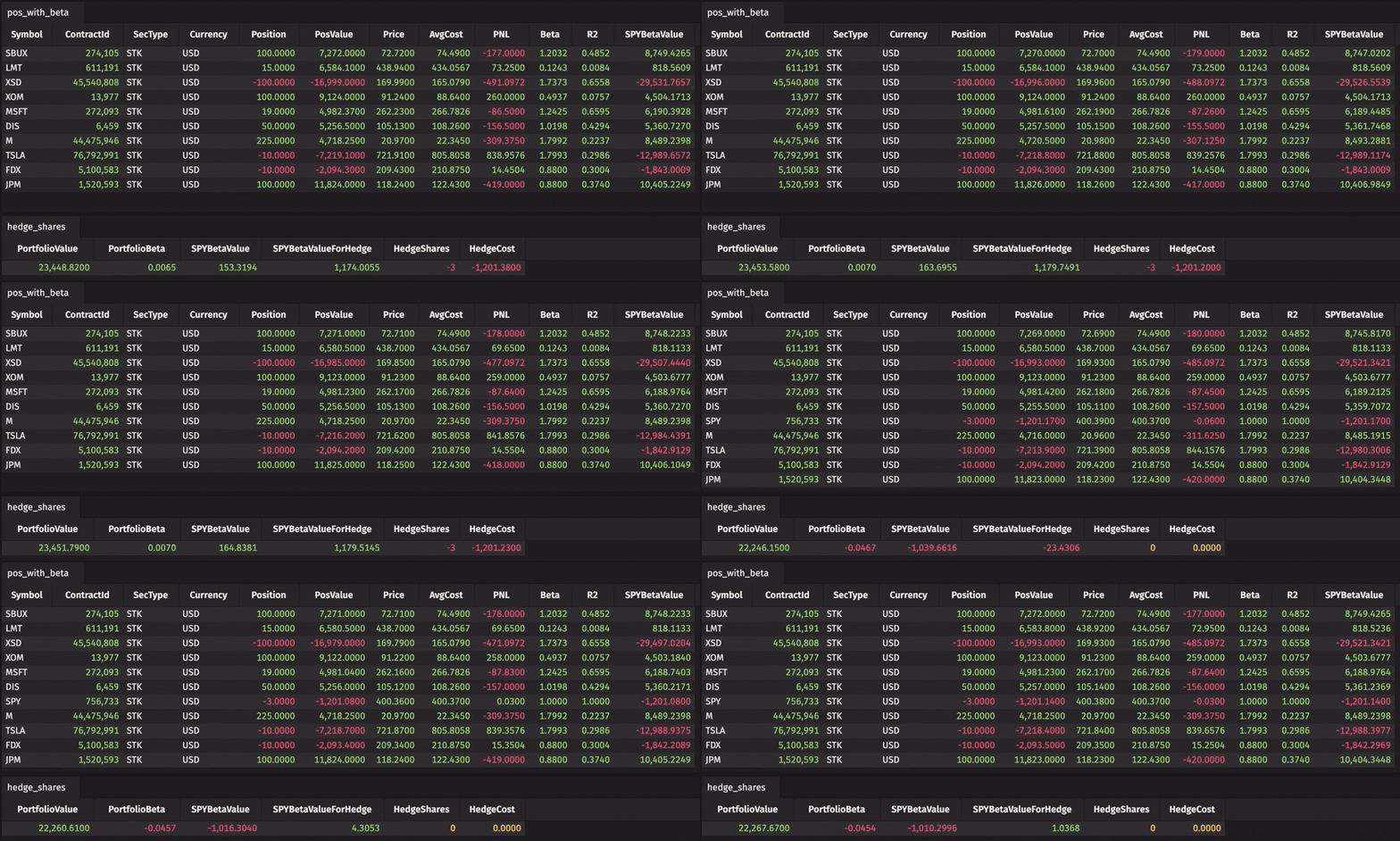
In the resulting hedge_shares table, we’ll be able to see our portfolio’s overall beta in the PortfolioBeta column,
our modeled SPY exposure in the SPYBetaValueForHedge, and the number of shares to trade to hedge that exposure in
the HedgeShares column.

As always in Deephaven, the results in the table will update dynamically as the source data changes — so we can monitor
the positions, prices, and risk as the market evolves throughout the day.

hedge_shares = pos_with_beta 
    .view([
        'PosValue',
        'WeightedBeta = Beta * PosValue',
        'SPYBetaValue',
        'SPYBetaValueForHedge = R2 > 1/3 ? SPYBetaValue : 0'
    ]) 
    .sum_by() 
    .natural_join(live_prices.where('Symbol=`SPY`'), [], ['SPY_Price=Price']) 
    .view([
        'PortfolioValue = PosValue',
        'PortfolioBeta = WeightedBeta / PosValue',
        'SPYBetaValue',
        'SPYBetaValueForHedge',
        'HedgeShares = -round(SPYBetaValueForHedge / SPY_Price)',
        'HedgeCost = HedgeShares * SPY_Price',
    ])

We’ve finished writing our beta hedge calculation query, so there’s only one thing left to do — make a trade!

The deephaven-ib plugin supports entering orders automatically, but for simplicity (and to avoid the risks of
automated trading), we’ll keep the API in read-only mode and enter the order manually.

The query recommends selling 3 shares of SPY, so let’s send the order:

When the order fills, “SPY” appears in our positions, and the rest of our calculations update — the portfolio beta,
recommended hedge, and position value. “HedgeShares” jumps down to zero shares, indicating that we are hedged to our
model’s satisfaction.

This is one example of how to monitor and hedge risk in Deephaven, but Deephaven’s inherent flexibility allows for
countless other variations. The simple workflow presented here can be adapted to different time horizons, benchmarks,
risk metrics, and hedging logic. Check out our documentation and
examples or reach out to us
on Slack to learn more!