Easy TensorFlow predictions using GPUs | Deephaven

The release of pip-installed Deephaven is a game changer for data scientists. This new way of connecting to a Deephaven server allows you to build and develop your projects locally in a Docker-less environment. Besides that, deephaven.learn can now harness the power of your GPU. To show this off, I’ve created an example using the learn package in conjunction with TensorFlow and my GPU.

The example project uses a simple neural network to recognize three different classes in the Iris-flower data set. We’ll see how this computation can be performed on your GPU.

Before following along with my sample code, go through the setup steps below.

1. GPU set up for WSL in Windows​

Follow the steps here to enable GPU accessibility in WSL. To check if the GPU is set up properly on your local machine, run:

For my computer, GeForce 3050 is my default GPU. We can see that the GPU usage is 0% at this point.

2. Deephaven Python package​

This is all it takes to install Deephaven:

pip3 install --upgrade pip setuptools wheel
pip3 install deephaven-server

With that out of the way, I’ll walk you through some of my data science workflows, such as deep learning projects using the deephaven.learn package, with GPU computation power.

We first import the packages, and build the server on port 10000, which allows us to access the Deephaven IDE there later:

from deephaven_server import Server
s = Server(port=10000, jvm_args=["-Xmx4g"])
s.start()

We can run this code to check if the GPU is accessible by TensorFlow:

import tensorflow as tf
gpus = tf.config.experimental.list_physical_devices('GPU')
for gpu in gpus:
    print("Name:", gpu.name, "  Type:", gpu.device_type)

If the GPU on your local machine is compatible with TensorFlow, it will print out Name: /physical_device:GPU:0 Type: GPU

Here we use the Iris data set, a very common data science data set for illustration. I did some data pre-processing to assign numeric classes to each flower category:

from deephaven import read_csv, new_table

iris_data = read_csv("https://media.githubusercontent.com/media/deephaven/examples/main/Iris/csv/iris.csv")
table2 = new_table([
    string_col("Class", ["Iris-setosa", "Iris-versicolor", "Iris-virginica"]),
    int_col("class_1", [0, 1, 2])
])
iris=iris_data.exact_join(table=table2, on=["Class"]).drop_columns(cols=["Class"]).rename_columns(cols=["Class=class_1"])

Here is the deep learning model I built for classification. More complex neural networks would require more GPU computational power, which you can see from the later picture. We also follow the typical modeling procedures to define optimizer, loss function and evaluation metrics in the train_model function.

model = Sequential()
model.add(Dense(512, input_shape=(4,), activation=tf.nn.relu))
model.add(Dense(256, input_shape=(512,), activation=tf.nn.relu))
model.add(Dense(128, input_shape=(256,), activation=tf.nn.relu))
model.add(Dense(64, input_shape=(128,), activation=tf.nn.relu))
model.add(Dense(32, input_shape=(64,), activation=tf.nn.relu))
model.add(Dense(16, input_shape=(32,), activation=tf.nn.relu))
model.add(Dense(3, input_shape=(16,), activation=tf.nn.softmax))


def train_model(features, targets):
    model.compile(optimizer=
        tf.keras.optimizers.Adam(learning_rate=0.001), 
        loss=tf.keras.losses.SparseCategoricalCrossentropy(from_logits=True), 
        metrics=["accuracy"])

model.fit(x=features, y=targets, epochs=5)

These functions are to make sure that the input and output values are the correct data types:

def predict_with_model(features):
    predictions = model.predict(features)
    return [np.argmax(item) for item in predictions]


def table_to_array_double(rows, cols):
    return gather.table_to_numpy_2d(rows, cols, np_type=np.double)


def table_to_array_int(rows, cols):
    return gather.table_to_numpy_2d(rows, cols, np_type=np.intc)


def get_predicted_class(data, idx):
return data[idx]

After all functions and values get defined, we simply call learn.learn for the first time to train the model, then we call it again to output the table with predicted values.

learn.learn(
    table=iris,
    model_func=train_model,
    inputs=[learn.Input(inps, table_to_array_double), learn.Input(["Class"], table_to_array_int)],
    outputs=None,
    batch_size=iris.size
)


iris_predicted_static = learn.learn(
    table=iris,
    model_func=predict_with_model,
    inputs=[learn.Input(inps, table_to_array_double)],
    outputs=[learn.Output("PredictedClass", get_predicted_class, "int")],
    batch_size=iris.size
)

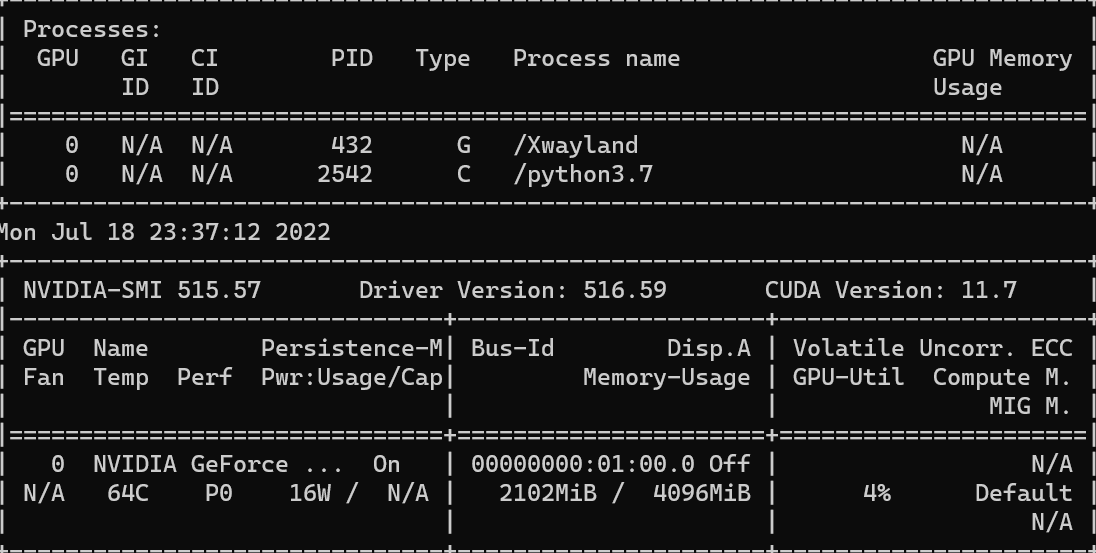
Now we see that the GPU usage goes up to 4%.

Navigate to http://localhost:10000/ide to access Deephaven IDE and you will see the iris_predicted_static table is already there.

Isn’t this cool? Think about how we can do it interactively. I prefer to do code editing on VS code, then after the script is executed, analyze and plot the results in the Deephaven IDE since it provides a better UI. What about you?

Feel free to start your own project by using Deephaven as a Python library, and contact us on Slack if you have any questions or feedback.