Exploring Probabilistic Search: The Power of the BM25 Algorithm

Home » Blog

Table of Contents

Exploring Probabilistic Search: The Power of the BM25 Algorithm

Probabilities in Search: The Probability Ranking Principle (PRP)

The Probability Ranking Principle (PRP)
Using Matching Score to Compute Relevance

The Okapi BM25 Algorithm

The BM25 Score
Connection between BM25 Score and Probability Ranking Principle

Inverse Document Frequency (IDF)
Term Frequency (TF)
Document Length Normalization

How to Build a BM25-Based Probabilistic Search for ArXiv Paper Abstracts

Step-by-Step Guide to Downloading the ArXiv Paper Abstracts Dataset
Loading and Preparing the ArXiv Dataset for Analysis
Constructing the BM25 Index
Performing a Search on a Sample Query

Summary

Citation Information

Exploring Probabilistic Search: The Power of the BM25 Algorithm

In this tutorial, you will learn about Probabilistic Search. Probabilistic search emerges as a powerful tool in the realm of information retrieval and web search. Unlike traditional semantic or Boolean search methods, which rely on exact matches or binary logic, probabilistic search takes into account the uncertainty and relevance of information. It assigns a probability score to each document in a collection, reflecting the likelihood of that document satisfying the user’s information need.

One such probabilistic model that has gained significant attention is the “BM25” (Best Match 25) algorithm. The BM25 algorithm, with its probabilistic foundation, offers a more sophisticated and effective approach, making it a compelling topic of exploration. This blog post aims to delve into the power of the BM25 algorithm, shedding light on its workings, its strengths, and its practical applications.

This lesson is the last in a 3-part series on unlocking the power of search: Boolean, semantic, and probabilistic search models explained.

To learn how Probabilistic Search works, just keep reading.

Exploring Probabilistic Search: The Power of the BM25 Algorithm

Probabilistic search models (e.g., the BM25 algorithm) offer several advantages over traditional vector space and Boolean models.

Handling Uncertainty: Probabilistic search models work by assigning a probability score to each document, reflecting the likelihood of that document satisfying the user’s query. This makes them capable of handling uncertainty and information relevance.
Term Independence: Vector space models assume term independence (i.e., each term is independent of its own and doesn’t affect the weighting of other terms in the document). This is often not true in practice, and probabilistic models offer a strategic way to handle dependencies between different terms.
Term Weighting: Probabilistic models, especially the BM25 algorithm, have shown very good performance in term weighting, which is crucial for effective information retrieval.

Probabilities in Search: The Probability Ranking Principle (PRP)

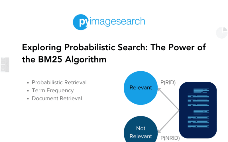
Probabilities provide a principled foundation for uncertain reasoning. So, can we use probabilities to quantify our search uncertainties? The idea is to rank by the probability of relevance (Figure 1) of the document w.r.t. the information we need.

**Figure 1:** The probabilistic search model works by assigning a probability score to each document in a collection, reflecting the likelihood of that document satisfying the user’s information need (source: SlideShare).

The Probability Ranking Principle (PRP)

The Probability Ranking Principle (PRP) is a fundamental concept in information retrieval that guides the ranking of documents in response to a user’s query based on probabilities.

To understand PRP in simpler terms, imagine you’re in a library full of books, and you’re looking for books on a specific topic, say “gardening.” Now, not all books in the library are going to be about gardening, and even among the gardening books, not all are going to be equally useful to you. Some might be too advanced, some might be too basic, and some might be just right.

The PRP is like a helpful librarian who can predict which books you’ll find useful. The librarian doesn’t just randomly give you books. Instead, they rank the books based on how likely each book is to be useful to you. The book that the librarian thinks is most likely to be useful to you is given first, then the next most likely, and so on. This is the essence of the PRP — it’s all about ranking items (like documents or web pages) based on their likelihood of being useful or relevant.

Now, how does the librarian (or the PRP) make these predictions? They use evidence and prior knowledge. Evidence could be the words used in your query and the words found in the document. Prior knowledge could be what the system already knows about the relevance of certain terms or documents.

In search engines, the PRP ranks the search results. When you type a query into a search engine, the search engine uses the PRP to predict which web pages you’ll find most useful or relevant (Figure 2) and shows you these pages first.

**Figure 2: The** Probability Ranking Principle guides the ranking of documents in response to a user’s query based on probabilities (source: SlideServe).

Using Matching Score to Compute Relevance

Suppose that the probability of relevance of an $i$ th document $d_i$ for a given query $q$ is given as:

$P(R= X | d_i, q)$

where $X in { 0, 1 }$ (1 denoting relevance, and 0 denoting irrelevance).

The matching score of a query-document pair can be written as the ratio between the probability of relevance and the probability of non-relevance of the document to the query:

$mathcal{M}_{d_i, q} = displaystylefrac{P(R= 1 | d_i, q)}{P(R= 0 | d_i, q)}$

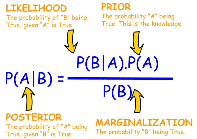
Using Bayes theorem (Figure 3), we can write:

$P(R= X | d_i, q) = P(R=X) cdot P(d_i | R=X, q)$

where:

$P(R=X)$ here is the probability that the document chosen at random (without any prior knowledge of its content) is relevant $(X=1)$ or non-relevant $(X=0)$ to the query.
$P(d_i | R=X, q)$ is the probability of choosing a document from a relevant $(X=1)$ or non-relevant $(X=0)$ set.

**Figure 3:** Bayes Theorem overview (source: Virginia Stoner Writing & Art).

With this, we can re-express the matching score as:

$mathcal{M}_{d, q} = displaystylefrac{P(R=1) cdot P(d_i | R=1, q)}{P(R=0) cdot P(d_i | R=0, q)}$

Since $P(R=X)$ is the same for all documents, we can ignore these from our equations and simplify them as:

$mathcal{M}_{d_i, q} propto displaystylefrac{P(d_i | R=1, q)}{ P(d_i | R=0, q)}$

To estimate the probabilities $P(d_i | R=1, q)$ and $P(d_i | R=0, q)$ , we need to see the distribution of query terms inside the document and inside the whole collection.

If we assume term independence, which means that the terms in the query $q$ appear independently of each other, we can write:

$P(d_i | R=1, q) = prod_{t in q} P(d_i | R=1, t)$

where $t$ is a term in the query. Using this, we can further simplify the matching score as follows:

$mathcal{M}_{d_i, q} propto prod_{t in q} displaystylefrac{P(d_i | R=1, t)}{ P(d_i | R=0, t)}$

Taking logarithms on both sides, we get:

$log(mathcal{M}_{d_i, q}) propto sum_{t in q} logleft(displaystylefrac{P(d_i | R=1, t)}{ P(d_i | R=0, t)}right)$

Thus, if we can compute the log-probabilities $logleft(displaystylefrac{P(d_i | R=1, t)}{P(d_i | R=0, t)}right)$ of how relevant a document $d_i$ is for a term $t$ in a given query, we can estimate the matching score $log(mathcal{M}_{d_i, q})$ which can be used to rank documents!

The Okapi BM25 Algorithm

BM25 is a ranking function used by search engines to rank matching documents according to their relevance to a given search query. It is based on the probabilistic retrieval framework. It is a bag-of-words retrieval function that ranks a set of documents based on the query terms appearing in each document, regardless of their proximity within the document.

The BM25 Score

The BM25 algorithm is an extension of the TF-IDF (Term Frequency-Inverse Document Frequency) method, which is a numerical statistic that reflects how important a word or term is to a document in a collection or corpus.

The BM25 algorithm looks at three main factors (Figure 4):

How often the query terms appear in the document.
The length of the document.
The average length of all documents in the collection.

The BM25 score of a document $d_i$ for a given query $q$ is calculated as follows:

$text{score}(d_i, q) = sum_{t in q} text{IDF}(t) cdot displaystylefrac{f(t, D) cdot (k_1 + 1)}{f(t, d_i) + k_1 cdot left(1 - b + b cdot displaystylefrac{|d_i|}{text{avgdl}}right)}$

where:

$t$ is a query term.
$f(t, d_i)$ is the term frequency of term $t$ in document $d_i$ .
$vert d_ivert$ is the length of document $d_i$ in words.
$text{avgdl}$ is the average document length in the text collection.
$k_1$ and $b$ are free parameters, usually chosen as $k_1 = 1.2$ and $b = 0.75$ .
$text{IDF}(t)$ is the inverse document frequency of the query term $t$ in the collection computed as:
$text{IDF}(t) = log left( displaystylefrac{N - n(t) + 0.5}{n(t) + 0.5} right)$

where $N$ is the total number of documents in the collection, $0.5$ is a smoothing constant, and $n(t)$ is the total number of documents containing term $t$ .

**Figure 4:** Different components of the BM25 similarity score (source: Medium).

Connection between the BM25 Score and Probability Ranking Principle

According to the probability ranking principle, the log-matching score is given by:

$log(mathcal{M}_{d_i, q}) propto sum_{t in q} logleft(displaystylefrac{P(d_i | R=1, t)}{P(d_i | R=0, t)}right)$

The matching score here depends on the following two quantities.

It is directly proportional to $P(d_i | R=1, t)$ , which measures how important a term $t$ is for a document $d_i$ . If we think carefully, this is similar to the term frequency of a term in a document which measures how frequently a term appears in a document.

It is inversely proportional to $P(d_i | R=0, t)$ , which measures how unimportant a term $t$ is for a document $d_i$ . This is similar to the inverse document frequency of a term in a collection, which measures how rare that term is in the collection.

The BM25 ranking formula is given by:

$text{score}(d_i, q) = sum_{t in q} text{IDF}(t) cdot displaystylefrac{f(t, D) cdot (k_1 + 1)}{f(t, D) + k_1 cdot left(1 - b + b cdot displaystylefrac{|d_i|}{text{avgdl}}right)}$

Let’s see how it connects to the matching score.

Inverse Document Frequency (IDF)

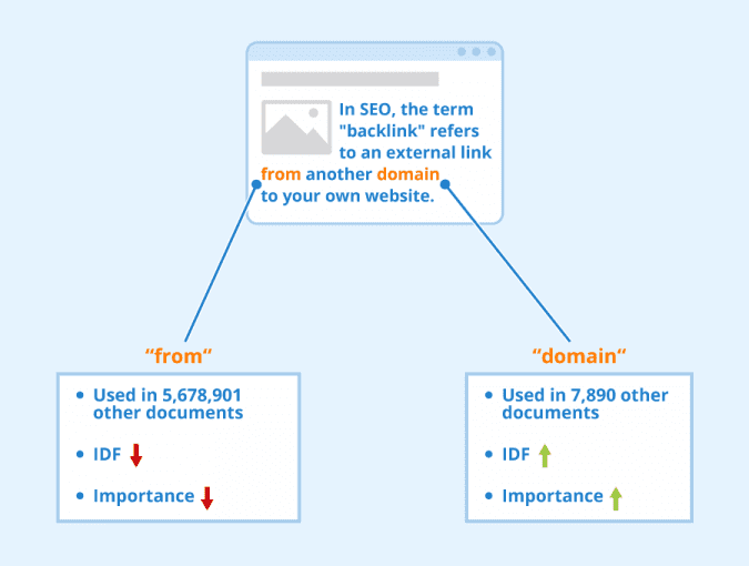
The $text{IDF}(t)$ term in the BM25 formula represents the informativeness of a term (Figure 5). It is derived from the matching score of a term appearing in relevant versus non-relevant documents. Mathematically, it can be expressed as:

$text{IDF}(t) = log left( displaystylefrac{N - n(t) + 0.5}{n(t) + 0.5} right)$

where ( $N$ ) is the total number of documents and $(n(t_i))$ is the number of documents containing term ( $t_i$ ). This term adjusts the weight of a term based on its rarity, aligning with the idea that rarer terms are more informative.

**Figure 5:** Inverse Document Frequency (source: Seobility Wiki).

Term Frequency (TF)

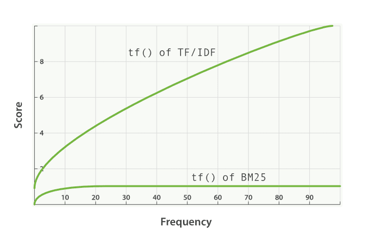
The term frequency $f(t, d_i)$ represents how often term $t$ appears in document $d_i$ . In the PRP matching score framework, higher term frequency increases the odds of relevance. The BM25 formula uses a saturation function to model diminishing returns of term frequency:

$displaystylefrac{f(t, d_i) cdot (k_1 + 1)}{f(t, d_i) + k_1}$

This term ensures that the impact of term frequency grows logarithmically, reflecting the intuition that each additional occurrence of a term contributes less to the relevance score (Figure 6).

The parameter $k_1$ controls the saturation of term frequency. It determines how quickly the term frequency effect saturates. A higher $k_1$ value means slower saturation.

**Figure 6:** Term frequency in standard TF-IDF versus Term frequency with saturation in BM25 (source: Elastic Blog).

Document Length Normalization

The term $displaystylefrac{|D|}{text{avg}|D|}$ , known as document length normalization, adjusts the term frequency to account for the length of the document. Longer documents are more likely to contain any given term simply by chance. The normalization factor is given by:

$1 - b + b cdot displaystylefrac{|D|}{text{avgdl}}$

where $b$ is a parameter (usually between 0 and 1) that adjusts the term frequency based on the document length relative to the average document length. This helps to prevent longer documents from being unfairly favored (Figure 7).

**Figure 7:** Importance of document length normalization in BM25 (source: SlideServe).

How to Build a BM25-Based Probabilistic Search for ArXiv Paper Abstracts

Now, let’s learn to implement a probabilistic search model on the arXiv paper abstracts dataset using the BM25 similarity score. The arXiv paper dataset consists of 50K+ paper titles and abstracts from various research areas.

The goal is to build a model that can retrieve relevant arXiv papers for a given free text query, such as: “machine learning for covid-19 using GANs.”

Step-by-Step Guide to Downloading the ArXiv Paper Abstracts Dataset

We will download our arXiv paper abstracts dataset using the Kaggle API. Here’s how you can install the Kaggle API and the arXiv dataset on your system:

$ pip install kaggle
$ kaggle datasets download -d spsayakpaul/arxiv-paper-abstracts
$ unzip <path-to-zip>/arxiv-paper-abstracts.zip -d /<path-to-data>/

Loading and Preparing the ArXiv Dataset for Analysis

Before loading our arXiv paper abstracts dataset, let’s install some important Python libraries that we will use in this project:

nltk: The Natural Language Toolkit (NLTK) is a comprehensive Python library that provides a suite of tools for tasks such as tokenization, stemming, lemmatization, part-of-speech tagging, and named entity recognition.
pandas: Pandas is a powerful, open-source Python library for data manipulation and analysis. We will use pandas to read and manipulate our datasets saved in CSV format.
numpy: NumPy is a popular Python library that supports large, multi-dimensional arrays and matrices, along with a large collection of high-level mathematical functions.
bm25s: A library that implements BM25 in Python, allowing you to rank documents based on a query. BM25 is a widely used ranking function for text retrieval tasks and a core component of search services like Elasticsearch.

Here’s how to install the required Python libraries using pip.

$ pip install pandas numpy nltk bm25s

Next, we will import these libraries into our Jupyter Notebook and load and visualize the dataset.

import numpy as np
import pandas as pd
from nltk.stem import PorterStemmer
from nltk.corpus import stopwords
import string
import bm25s

import nltk
nltk.download('stopwords')

from IPython.display import display, HTML

data = pd.read_csv("/<path-to-data>/arxiv_data.csv", header="infer")
print("Total rows : ", len(data))

display(HTML(data.head().to_html()))

On Lines 1-8, we import the pandas, numpy, nltk, and bm25s libraries. Next, on Line 9, we download the list of stopwords from the nltk package.

On Lines 13-16, we load the arxiv_data.csv using the pandas.read_csv() utility. We print the number of rows in the dataset and also visualize some of them using the IPython display. Figure 8 displays the output of the above code block.

**Figure 8:** Snapshot of an arXiv paper abstracts dataset (source: arXiv Paper Abstracts on Kaggle).

Each row in the dataset has three fields:

titles: The title of the research paper.
summaries: The abstract of the research paper.
terms: The tags associated with the paper.

Constructing the BM25 Index

Next, we will construct the BM25 index over the whole corpus of arXiv abstracts.

stemmer = PorterStemmer()
stop_words = set(stopwords.words("english"))

corpus = []

for summary in data.summaries.to_list():
  tokens = summary.lower().split()
  # Stemming and stop-word removal
  tokens = [stemmer.stem(token) for token in tokens if token not in stop_words]
  corpus.append(" ".join(tokens))

print(corpus[0])

retriever = bm25s.BM25(corpus=data.index.tolist())
retriever.index(bm25s.tokenize(corpus))

Let’s understand the above code snippet line-by-line.

On Lines 18-29, we perform basic preprocessing steps on the arXiv abstracts. For each summary in the data.summaries list, we split the summary into lowercase tokens (words). After that, we apply stemming and stop-word removal where each token is stemmed (reduced to its root form) using the Porter stemmer, and stop words (common words like “the,” “and,” etc.) are removed. The processed tokens are joined back into a single string and added to the corpus.

On Lines 31 and 32, we initialize a BM25 model retriever using a corpus created from the index of a DataFrame. Next, we tokenize this corpus and index it, enabling the BM25 model to retrieve and rank documents based on search queries efficiently.

Performing a Search on a Sample Query

So far, we have processed our text data and created a BM25 index. The code snippet below shows how to perform a search for a sample query using this BM25 index.

TopK = 10

# Query the corpus and get top-k results
query = "machine learning for covid-19 research using segmentation"
doc_indices, scores = retriever.retrieve(bm25s.tokenize(query), k=TopK)

# Display the relevant documents
titles = []
abstracts = []
similarity = []
for doc_index in doc_indices[0]:
  titles.append(data.iloc[doc_index].titles)
  abstracts.append(data.iloc[doc_index].summaries.replace("n", " "))

results = pd.DataFrame({"Title": titles, "Abstract": abstracts, "Similarities": scores[0]} )
display(HTML(results.to_html()))

Let’s understand the above code snippet line-by-line:

On Line 34, we also define the TopK variable that specifies the number of relevant documents to retrieve.

On Lines 37 and 38, we define a sample query: "machine learning for covid-19 research using segmentation". The query is then first tokenized (using bm25s.tokenize) and then passed through the BM25 retriever to retrieve TopK document indices (doc_indices) and their corresponding BM25 scores (scores).

On Lines 40-49, for each relevant document ID in doc_indices, the title and abstract are extracted from the original dataset (data). The results are displayed in a Pandas DataFrame, including columns for the title, abstract, and BM25 similarity score.

Figure 9 displays the result of the above code snippet.

**Figure 9:** Output for BM25-based probabilistic search (source: image by the author).

As you can see from the output, for our sample query, "machine learning for covid-19 research using segmentation", the BM25-based semantic search can retrieve and rank documents based on their relevance.

Summary

In this blog post, we delve into the intricacies of probabilistic search models, focusing on the BM25 algorithm. We begin by introducing the concept of probabilistic search and the Probability Ranking Principle (PRP), which is fundamental to understanding how search engines rank documents based on their relevance to a query. We explain the PRP in detail, highlighting its role in computing relevance scores using matching scores.

We then transition to a comprehensive discussion of the Okapi BM25 algorithm, a widely used probabilistic model in information retrieval. We explain the BM25 score and its connection to the PRP, emphasizing how the algorithm leverages Inverse Document Frequency (IDF) and Term Frequency (TF) to rank documents. We also cover the importance of document length normalization in refining search results, ensuring that longer documents do not unfairly dominate the rankings.

In the practical section, we provide a step-by-step guide to building a BM25-based probabilistic search system for arXiv paper abstracts. This includes instructions on downloading the arXiv paper abstracts dataset, preparing it for analysis, and constructing the BM25 index. We conclude with a demonstration of performing a search on a sample query, showcasing the effectiveness of the BM25 algorithm in retrieving relevant documents.

Citation Information

Mangla, P. “Exploring Probabilistic Search: The Power of the BM25 Algorithm,” PyImageSearch, P. Chugh, A. R. Gosthipaty, S. Huot, K. Kidriavsteva, and R. Raha, eds., 2024, https://pyimg.co/xb6cm

@incollection{Mangla_2024_Exploring-Probabilistic-Search-BM25-Algorithm,
  author = {Puneet Mangla},
  title = {Exploring Probabilistic Search: The Power of the BM25 Algorithm},
  booktitle = {PyImageSearch},
  editor = {Puneet Chugh and Aritra Roy Gosthipaty and Susan Huot and Kseniia Kidriavsteva and Ritwik Raha},
  year = {2024},
  url = {https://pyimg.co/xb6cm},
}

Join the PyImageSearch Newsletter and Grab My FREE 17-page Resource Guide PDF

Enter your email address below to join the PyImageSearch Newsletter and download my FREE 17-page Resource Guide PDF on Computer Vision, OpenCV, and Deep Learning.

The post Exploring Probabilistic Search: The Power of the BM25 Algorithm appeared first on PyImageSearch.

Source link
lol

Exploring Probabilistic Search: The Power of the BM25 Algorithm – PyImageSearch

Exploring Probabilistic Search: The Power of the BM25 Algorithm

Exploring Probabilistic Search: The Power of the BM25 Algorithm

Probabilities in Search: The Probability Ranking Principle (PRP)

The Probability Ranking Principle (PRP)

Using Matching Score to Compute Relevance

The Okapi BM25 Algorithm

The BM25 Score

Connection between the BM25 Score and Probability Ranking Principle

Inverse Document Frequency (IDF)

Term Frequency (TF)

Document Length Normalization

How to Build a BM25-Based Probabilistic Search for ArXiv Paper Abstracts

Step-by-Step Guide to Downloading the ArXiv Paper Abstracts Dataset

Loading and Preparing the ArXiv Dataset for Analysis

Constructing the BM25 Index

Performing a Search on a Sample Query

Summary

Citation Information

Join the PyImageSearch Newsletter and Grab My FREE 17-page Resource Guide PDF

By stp2y

Leave a Reply Cancel reply